GC Image GCxGC Edition Users' Guide

Introduction

GC Image GCxGC Edition is a system designed for visualizing, processing, analyzing, and reporting on data produced in two-dimensional gas chromatography (GCxGC). GC Image GCxGC Edition has three main interfaces:

GC Image
GC Project
Investigator

This introduction provides a brief overview of GCxGC data and a quick tour of some of the image processing facilities of GC Image GCxGC Edition. Chapter 2 contains installation instructions for the software. Chapters 3-17 describe the GC Image interface and chapters 18-20 describe GC Project. Chapters 21-22 contain instructions for calibration and reporting. Chapter 23 introduces the Help Resources for the software. Appendix A provides Answers to Frequently Asked Questions . Appendix B is a white paper on GCxGC Blob Metadata and Statistics in GC Image. Appendix C describes the plugin interface for the software.

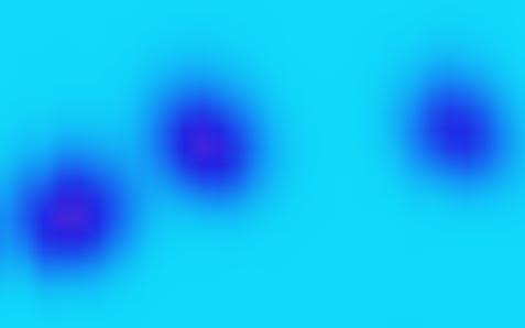
GCxGC separates chemicals according to the time each chemical requires to pass through two capillary columns. GCxGC data can be displayed as an image with pixels arranged so that the abscissa (X-axis) is the retention time for chemicals to pass through the first column and the ordinate (Y-axis) is the retention time for chemicals to pass through the second column. Each pixel value indicates the rate at which molecules are detected at a specific time.

The elution of a compound(s) in the sample produces a small blob or cluster of data-point pixels with values that are larger than background values. The magnitudes of the data-point pixel values indicate the quantity of the chemical(s) present. fig.threeBlobs illustrates a greatly magnified view of a small region of a GCxGC image containing three blobs of pixels indicating (at least) three separated chemicals. The smaller values of the background are colorized light-blue and the larger values of the blobs are colorized dark-blue and magenta.

fig.threeBlobs: A region of a GCxGC image containing three blobs of pixels indicating three separated chemicals.

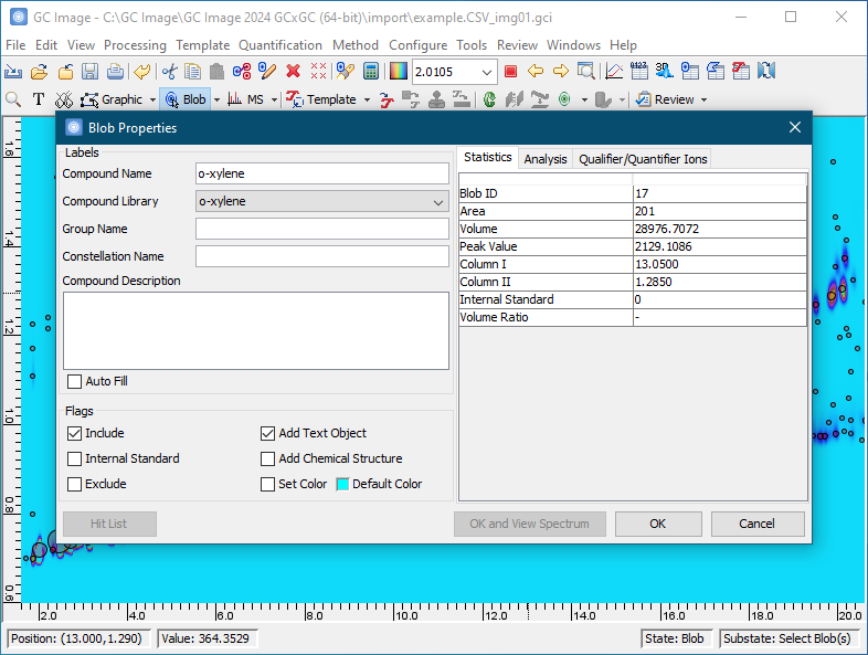
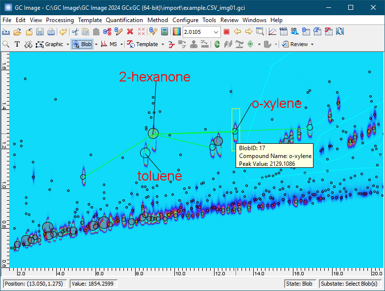
The position (i.e., the retention times in each dimension) of each blob is related to the physical properties the chemical(s) that produced the blob, so the position of a blob is useful in identifying each chemical in a sample. The sum of the pixel values in each blob is related to the quantity of the chemical that produced it, so the sum of pixel values of a blob is useful in quantifying the amount of each chemical in a sample.

Quick Tour

GC Image has many tools that support various operations. This quick tour illustrates some of the steps in a typical processing sequence to analyze raw data produced by GCxGC, identifying and quantifying chemicals in a sample:

Import a raw data file to create a chromatographic image.
Remove the background or baseline level from the chromatogram.
Detect the blob peaks in the chromatogram.
Identify and characterize the chemical compounds for the blob peaks.
Save the processed chromatogram and related metadata.

The following figures illustrate each of these steps. Later sections of the GC Image GCxGC Edition Users' Guide describe these and other operations in greater detail.

Step 1a: Click the Import Image button on the tool bar (a tool tip is shown) or select File -> Import Image from the menu.

Import Image Menu

Step 1b: For the Import Image operation, GC Image presents a file chooser to locate the source file with the chromatographic data.

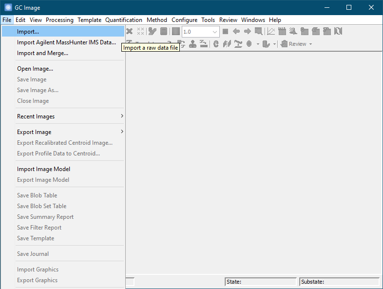
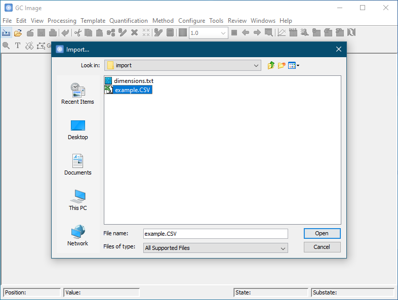
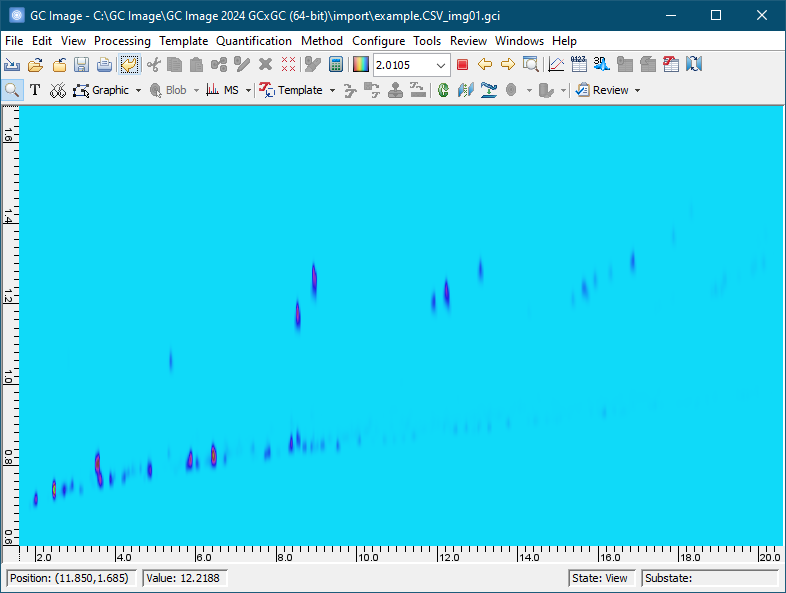
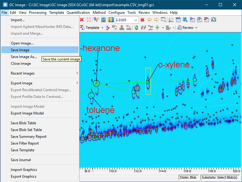
Locate the desired source data file and click the Open button. For example, a source file containing the raw chromatographic data can be a text file in comma-separated-value (CSV) format. The destination file name is automatically generated by GC Image, but can be changed by the user during the save operation.

Browse Source File

Step 1c: After GC Image accepts the filename, it presents a popup dialog box for additional information about the image dimensions and processing.

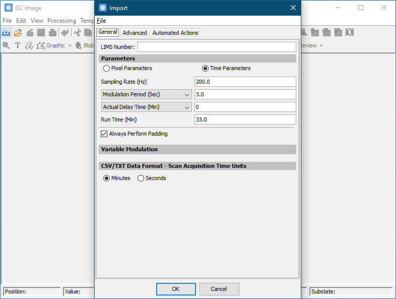
Specify the dimensions and optionally specify other processing options. The dimensions of the data are required and will be read from the source file if provided by the file format or may be specified by the user in pixel or time units. For example, the dimensions of data acquired at 200 Hz with a modulation period of 3 seconds and a run time of 33 minutes could be sized equivalently as 660 pixels for the first dimension (33 minutes / 3 seconds / modulation) and 600 pixels for the second dimension (200 samples/second * 3 seconds).

Specification of a configuration file and processing operations are optional in this pop-up. These optional specifications are a convenient mechanism for quickly directing processing at the time data is imported. Chapter Configurations describes these capabilities. The rest of this quick tour demonstrates how the processing operations are performed interactively.

Import Dialog

Step 1d: After the data is imported to form a chromatographic image it is displayed in the Image Viewer. A magnified region-of-interest (ROI) is shown below. Here and in other figures, the GC Image interface is resized to a small window for tutorial presentation.

ROI in Image Viewer

Step 1e: Select View > Colorize from menu to adjust the color map to reveal details of the image.

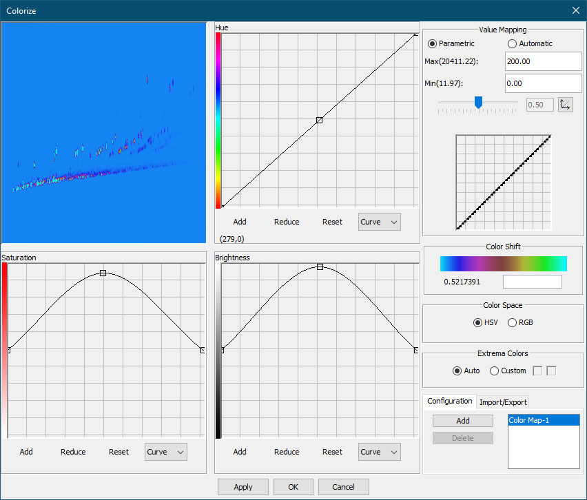
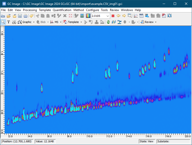
In the Colorize tool, set Max to 200 and Min to 0 under Value Mapping. Click OK to apply the new color map.

Colorize Tool

Step 1f: After the color map is adjusted more peaks are visible in the ROI as shown below.

ROI with Customized Color Map

Step 2: This image has a background level of over 12 pico-amps per data-point pixel in the chromatographic image. (See the status bar below the image with the location of the cursor and the data value at that pixel.) Before quantifying the blobs, the baseline must be corrected.

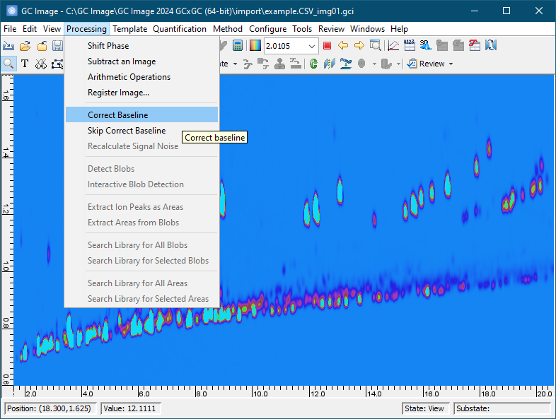
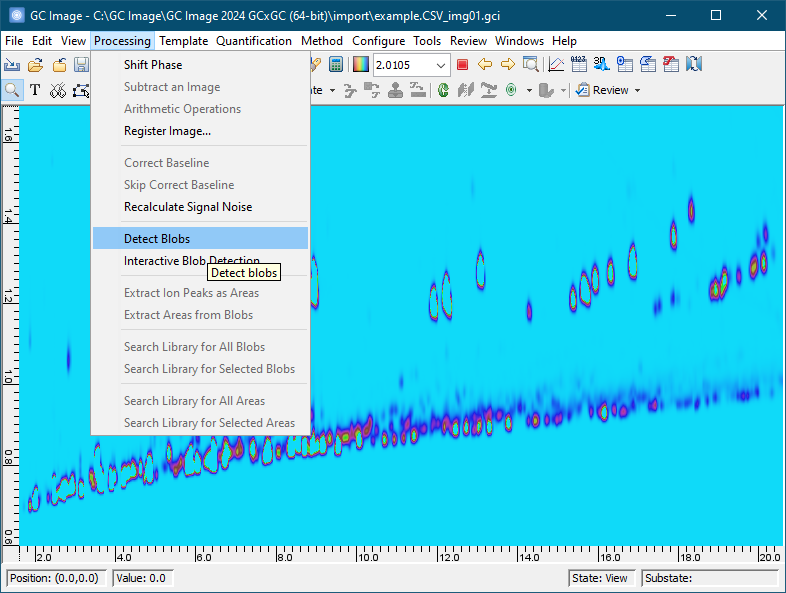
Click the Correct Baseline button on the tool bar (a tool tip is shown) or select Filter -> Correct Baseline from menu.

Correct Baseline

Step 3: After the baseline is corrected, note the change in background value (indicated by the color change and by the value on the status bar). Now, the blobs associated with the separated chemicals can be detected and quantified. Press the Detect Blobs button on the tool bar or select Filter -> Detect Blobs from menu.

Detect Blobs

Step 4a: The blobs are detected and graphically highlighted by a bubble, thin outline, or other user-selectable highlight. An image may have thousands of blobs, but an analysis may require only a few of them. Later sections of the GC Image GCxGC Edition Users' Guide explain how to use template pattern matching to automatically identify and characterize peaks of interest. Here, the quick tour shows interactive identification and characterization.

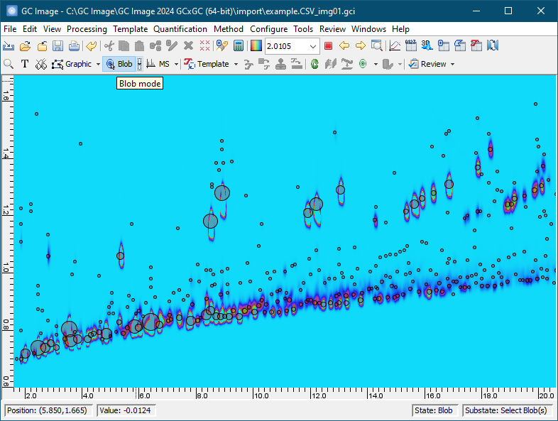
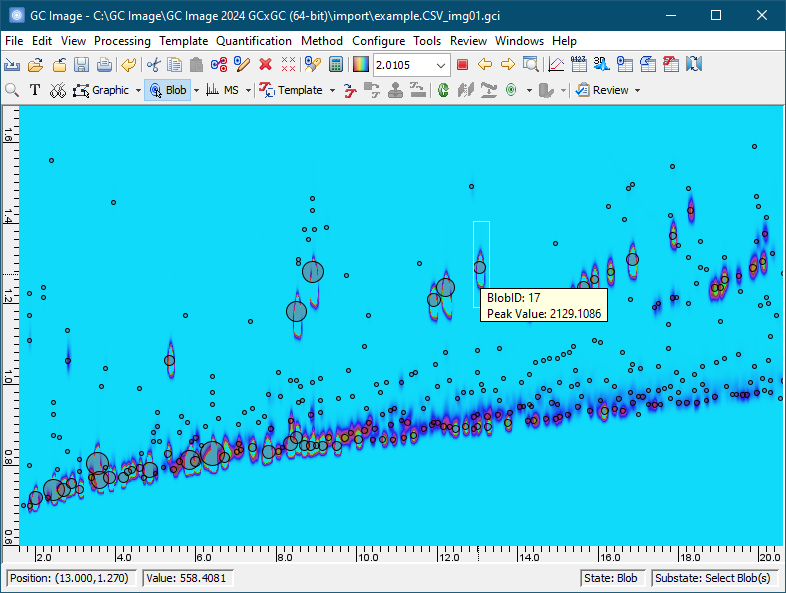
To select blobs for inclusion, first set the cursor mode on the Image Viewer palette to Blob Mode -> Select Blobs.

Blob Mode

Step 4b: Select a blob by positioning the cursor on the blob and clicking the left mouse-button. The selected blob is graphically highlighted with a colored box.

Select Blob

Step 4c: Once a blob is selected, click the right mouse-button to access a popup to view blob attributes and set blob metadata, including chemical name, group name, etc.

Edit Blob Properties

Step 4d: Graphical highlights show the included blobs, internal standards, associations between included blobs and internal standards, and other information.

Included Blobs with Internal Standard

Step 4e: To view the Blob Table, click the Show Blob Table button on the tool bar or select View -> Blob Table the menu. The Blob Table displays information about each blob. The table can be sorted by clicking on a column header and many other actions are supported.

Blob Table

Step 5: To save the chromatographic image and related metadata, click the Save Image button or select File -> Save on the menu. Then, exit by selecting File -> Exit from the menu.

Save Image

Subsequent chapters of the GC Image GCxGC Edition Users' Guide describe installation and details on using the software.

Contents Next: Installation and Start-Up