Multi-Sample Analysis - Wine GC-MS Peak Tables - Quick Start

Download sample data and get started using MDC Investigator/Analysis Software.

Step 1: Download Peak Tables

1. Download the sample peak tables:

   Sample Peak Tables

2. Unzip the downloaded peak tables (Right click on SamplePeakTables.zip and click Extract All…).

Step 2: Import Peak Tables

1. Launch the Analysis software.

2. From the File menu, select Load Images from Peak Tables….

3. Navigate to the location where you unzipped the peak tables. Use shift-select to select all the peak tables and click Open.

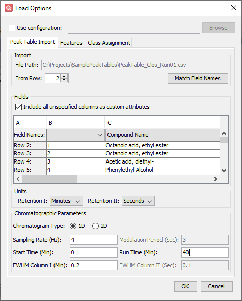
4. Configure settings on the Peak Table Import tab
   • Click Match Field Names to automatically fill the Field Names selection below.
   • Click Include all unspecified columns as custom attributes.
   • Set the Chromatogram Type to 1D.
   • Enter a Sampling Rate (Hz) of 4 and a Run Time (Min) of 40.
     
     
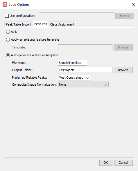
5. Configure settings on the Features tab
   • Click Auto generate a feature template.
   • Enter SampleTemplate as the File Name.
   • Click Browse beside the Output Folder field, navigate to your preferred save location, and click Save.
     
     
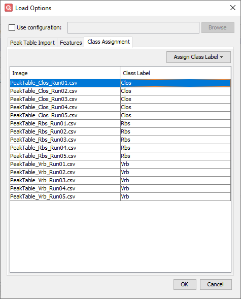
6. Configure settings on the Class Assignment tab
   • Use shift-select to select all PeakTable_Clos_Run##.csv files.
   • Click Assign Class and New Label.
   • Enter Clos for the class label and click OK.
   • Repeat this process to assign class Rbs to all PeakTable_Rbs_Run##.csv files and Vrb to all PeakTable_Vrb_Run##.csv files.
     
     

   

   

   

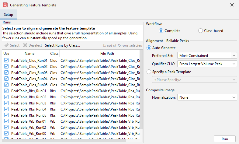
7. Click OK and get the Auto Feature configuration dialog.

   

8. Click Run and wait for feature template generation to complete. This will take some time (about 5-10 minutes).

9. Click OK and wait for the peak tables to import.

Step 3: Check Imported Data

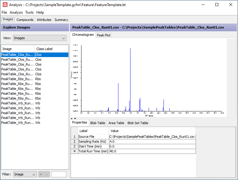
1. The list of imported images is shown on the right side of the window. It lists the image names and associated classes. Select PeakTable_Clos_Run01.csv.

2. Click the Chromatogram tab in the upper half of the window. This displays an estimate of the source chromatogram which produced the peak table.

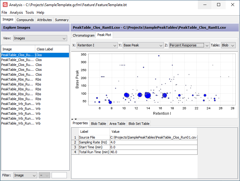
3. Click the Peak Plot tab in the upper half of the window. This displays configurable bubble plots of the data in the Peak Table and Area Table. Set the X axis combo box to Retention I, the Y axis combo box to Base Peak, and the Z axis combo box to Percent Response.

   

   

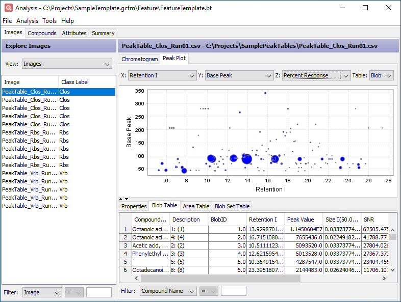
4. Click the Peak Table tab in the lower half of the window. This table contains the original data imported from the peak table. The added Description column indicates which feature area the peak belongs to.

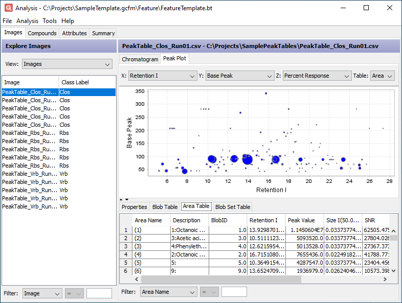
5. Click the Area Table tab in the lower half of the window. This table contains the peak table data restructured to support cross-sample analysis using the computed feature areas. Each row corresponds to a feature area. The values within that row come from the largest peak (by Peak Value) contained in the feature area. The added Description column indicates which peak is reported by the feature area.

   

   

Step 4: Perform PCA

1. From the action toolbar on the upper-right, click the Run PCA button.

2. On the Configure dialog that appears, select Areas as the Compound Type and Percent Response from the Attribute Selection list. Click OK.

3. Initially, PCA will not run due to missing values. First, configure the following:
   • At the bottom of the table, use the Filter to filter the table to the most relevant features. Set the first combo box to F Value, the second combo box to >, and the value field to 5.
   • Click the settings gear button on the upper-right of the PCA chart.
   • Set the Normalization combo box to Normalize by Feature and the Replace missing values with combo box to Zero (0). Click OK.
     
     

4. Click the Run PCA button on the upper-right of the PCA chart.

5. Change the Y axis combo box to PCA 4 to better separate the classes.